
During July 2020, the AFMBiomed summer school series was supposed to take place in Marseille, France. Due to CoVID travel restrictions, the course took place online. However, since, there was no travel involved, and because the organizers kindly decided to make signup free, the school, had a record number of participants. At times 300 people were online, which is amazing for a specialized course like this, and showed just how many people around the world want to learn about and improve their AFM!

The lecturers were really great, and despite working in this field for 20 years, even I learned some things! Since I thought the material was so good, I am including links to the archived lectures below. The "tutorial" lectures were particularly good. Note that although the overall topic was "Biomedical Science", there are techniques here that could be useful for any AFM user.
This link contains the lectures in .pdf format: https://amubox.univ-amu.fr/s/rtXJTnXZmsBc6XQ
Here You can find many of the lectures posted as videos on this site: https://zenodo.org/communities/afmbiomed?page=1&size=20
I highlight here some of the video tutorials that I found really useful:
- Nicolas Buzhinsky; - Mica surface preparation - especially for liquid applications: https://zenodo.org/record/3957408#.X1n5RHlKiUk
- Fidan Sumbul, Claire Valotteau and Felix Rico; - Cantilever and coverslip cleaning and surface coating methods and tips: https://zenodo.org/record/4017765#.X1n43HlKiUk
- Jean Luc Pellequer and Felix Rico; - Calibration of AFM cantilevers and optical response for force spectroscopy: https://zenodo.org/record/4005520#.X1n5r3lKiUk
Please note that these video are published with a DOI record, therefore, it would be helpful to the authors if you cite them. I found this online class really great, and hope it returns!
- Details
- Hits: 4101
I recently wrote an application note on using AFM to characterize two-dimensional materials for AFMWorkshop. The full article can be found here. What follows is a brief extract.
Two dimensional materials are currently under development with potential to gain enormous importance in electronics, sensing, optics and other areas. Such materials, despite facile production methods in many cases, can display radically different properties compared to 3D or bulk materials. These new and enhanced properties come about due to nanoscale confinement effects, meaning they are generally accessible only when a material is limited to one, or at most to a few atomic layers. For this reason, research and development in 2D material and 2D materials-based devices relies crucially on the ability to characterise such materials at the nanoscale, including the observation of atomic steps. Atomic Force Microscopes are ideally suited for creating 3-D images and measurements on 2-D materials. This is because AFMs have extreme contrast on flat samples and can magnify surface heights by factors of millions to billions. AFM is unique in its ability to measure sample heights with resolution in excess of 0.1 nm. This explains why AFM has become a key tool in the arsenal of researchers studying 2D materials - for example, see the two images of layered materials below.
 |
 |
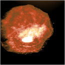
Figure 1a: Three dimensional color scaled image of SiC. The steps on this sample are 750 picometers.
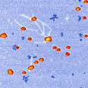
Figure 1b: Colourscale image of HOPG, showing atomic steps.
Besides illustrating the power of an AFM, these types of samples serve as calibration samples for microscopes used for imaging 2-D materials.
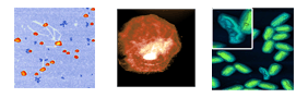
Graphene is an extraordinary new two-dimensional material, consisting of single atomic layers of sp2 carbon. Although graphene is a single atom thick sheet, it is not typically found to be perfectly flat. Indeed, some nanometre scale corrugations, are commonly observed and may increase the stability of the 2D lattice. Despite its great strength, graphene is also a highly flexible material, and typically takes on the form of the underlying substrate. So, for example, on Si/SiO2 wafers, graphene can exhibit a considerable roughness due to the underlying substrate. Thus, a considerable texture, dependent on the SiO2 structure at the wafer surface, can be seen in the CVD graphene flakes shown in the left image in figure 2 below.

Figure 2. Examples of AFM images of CVD graphene deposited on Si/SiO2 wafers. Left: Single-layer graphene on a silicon wafer. In this example, the effect of the underlying texture on the graphene sheet is clearly seen. Right: Multilayer graphene of a silicon wafer. Arrows highlight some wrinkle-like defects, typical of CVD graphene.
To read more about AFM applications to two-dimensional materials, read the full application note here.
- Details
- Hits: 2947
The last few years have seen quite a few changes in the AFM industry with some companies disappearing, and some others being acquired. presumably some caused by the financial crisis, which has certainly affected instrument spending.
Nanotec, a small Spanish company ceased trading in 2015. Nanotec were well-known for also producing their analysis software WSxM, which in addition to running their instruments, also opened almost all AFM image formats, and had a lot of great analysis features. Fortunately, WSxM is still available.
Keysight was a spin off of Agilent, and hosted the AFM division for a few years. unfortunately, they no longer make AFMs. Agilent had bought the IP of Molecular Imaging, which was one of the "big three" at one point. Agilent did continue to develop MI instruments for a number of years. Agilent had also bought the IP of Pacific Nanotechnology, but never did anything with it.
The biggest recent change is probably that Bruker bought JPK. JPK were early leaders in successful biological AFMs, and sold particularly well in Europe. As of now, Bruker are offering some of JPK's products and www.jpk.com still exists. I kind of hope this continues as their Nanowizard AFMs are good products. Bruker also bought Anasys instruments, which make Nano-infrared microscopes, and are now offered under the Bruker brand.
Asylum Research was acquired by Oxford Instruments, and are still trading under the name Asylum Research - An Oxford Instruments company.
Of course, in addition, a few smaller companies came and went as usual! All these changes are reflected in the page "Where to Buy - AFM Instruments", linked below.

I also link below to an interesting Post on LinkedIn from Paul West on the history of the AFM business, for those who are interested!
- Details
- Hits: 5358
Update
- Unfortunately, due to the coronavirus pandemic, we were unable to run the course on the proposed dates, so it's been postponed indefinitely.
Please click the image below to download the flyer with more details.

A blog with information and student feedback from the previous courses can be seen here:2017 course, 2014 course, 2013 course, 2011 course.
The course is supported by AFMWorkshop, The Faculty of Sciences of The University of Porto and my research institution, LAQV/Requimte.
- Details
- Hits: 18663
This is the second part of this article about how to write an academic paper including AFM data. If you have not already, you should read the first part here.
NOTE: Some of this content is not really specific to AFM articles, but could be applied to any experimental scientific report. These parts should already be known to you if you are writing an scientific article, but many researchers are never taught how to correctly prepare a scientific article before they start writing them. For more general guides on preparing scientific articles, check here.
Figure legend. The figure legend is an important part of the figure. It should not be too brief, e.g. “Figure 1. AFM images of samples 1 and 2.”. But it should also not be too long. It should be concise, but has to have all the information needed to enable the reader to understand the figure. It should have a description of the type of data, if necessary explain the scale of the images, and clearly identify the samples shown. For example, a good figure legend might be: “Figure 1. Representative tapping mode AFM images of samples 1 and 2. A: Height image of sample 1; B: Phase image of sample 1; C: Height image of sample 2; D: Phase image of sample 2. All images show 1????m x 1????m areas, and the z scales are indicated next to the height images. The arrows show the location of anomalous nanoparticles discussed in the text.”
-
Reproducibility
All numeric values included in the results must be accompanied by standard errors, or standard deviation of the means. You must also say how many measurements were made. It is important to discuss how many areas were imaged, and how often the features discussed in the text occurred. It’s not acceptable to show only one image, with the assumption that it represents a whole sample!
-
Conclusions
It should go without saying that the conlcusions you make based on your AFM data must be justified. This often means that you should calculate the occurrence of specific features, so if you want to say that the surface got rougher, or features grew after treatment, you should measure this, and show means, and errors, or a histogram of results. Note that histograms can help a lot with non standard data distributions, i.e. where there are outliers.
Can lateral measurements be used in AFM? Yes - but with caution, and only sometimes. If you have samples that are small, comparable to an AFM probe tip, lateral measurements of them will be wildly erroneous with AFM. For this reason it’s nearly always preferable to use vertical measurements where possible. Lateral measurements typically only work well for features much larger than the AFM probe, so you must be careful with these. One way to reduce the effect of these errors is to deconvolve the probe shape from your images. See section 2.3.4 of Atomic Force Microscopy.
If your conclusions are based on certain small features in your images, you can present your images in a way so as to make these features clear. This can be done by:
-
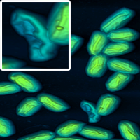
Cropping. A nice way to highlight certain features is to show a large image as well as a cropped section magnifying the feature you wish to show.
-
Histogram control. Control the height range shown in your height images to highlight the part you are interested in showing. So for example, if you wish to show tiny 20 nm features, you cannot do it with a z-scale of microns in a height image.
-
Shading. Light shading is a routine available in all AFM processing packages (such as SPIP and Gwyddion), which can highlight small topographic differences
-
Including error signals or phase images. These channels are frequently better for showing small details.
-
Highlighting with arrows. As discussed above.
-
Using unusual colour schemes. In general complex colour schemes make for confusing images, but for some images they can be appropriate, and help to illustrate the different features at different heights.
Some examples of these schemes are shown below.
Good luck with your AFM articles! If you have more questions, contact me here.
NB. All the images in these two articles were produced with SPIP 6.7.7 or Gwyddion 2.40
This article and all content is copyright Peter Eaton and AFMHelp.com 2019.
- Details
- Hits: 7026
Subcategories
Page 3 of 21